Here is a direct link to Snap!

To play with Snap! you can just click on the play button on some of the images, like the one above. If you have any problems with it loading, visit Snap! directly in a new browser tab (On that page, click "Run Snap! now"). Another possible solution, if your browser is not Chrome, is to give Chrome a try.

Graphs

In Class 8 we learned about a kind of data structure called Tree. Recall that a tree is made up of nodes and links. Also remember that a tree needs to have a root node, that is, a single node which has links to some other nodes and through those children nodes to all nodes in the tree. Other than the root nodes children, no other nodes can have a link back to the root node. Also links cannot create a cycle, meaning you cannot start from a node and follow the path of links back to itself.

A Graph is a another example of a data structure, where these restrictions are lifted. A Graph is a set of nodes and links, without any restriction of how many links exist and which nodes they connect. For a graph a node is more commonly called a vertex, and a link is called an edge. For example, here is a sample graph, with 11 vertices and 14 edges:

As you see, unlike a tree where there is a special node called the root, no vertices in a graph is more special than the others. It is also possible for a vertex to have no edges connecting to it, as the above graph also demonstrates.

It is common to have either the vertices, or the edges, or both, to represent values. For example, here is a graph which assigns a numeric value to each edge, but not to vertices:

Directed Graphs

In a Directed Graph the edges can optionally be "one-way" only, indicated by an arrow, rather than just a line. For example, here is a directed graph which has numeric values for both edges and vertices:

A Directed Graph indicates some sort of flow. For example, in the graph above, from vertex with value 2 we can only move to vertex labeled s or one with value 4.

Sometimes a graph can have a Start vertex, representing the starting point for the flow. That is what the label s is indicating in the above graph.

Shortest-Path Algorithm

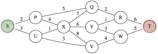
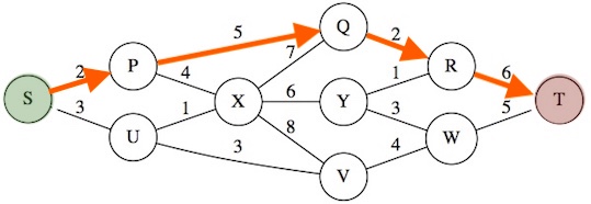
Imagine the vortices in this (undirected) graph above are modeling cities, and the numbered (aka, weighted) edges tell us the distance between those cities.

Imagine we want to travel from vertex labeled S ("source") to vertex labeled T ("target"). It is an interesting question to ponder "Which path is the shortest path from S to T?" This is called the Shortest-Path Problem.

There is an algorithm called the Shortest-Path Algorithm (or Dijkstra's Algorithm, named after the famous computer scientist.) to solve this problem for any arbitrary graph.

Remember than an algorithm is a set of concise, step by step instructions to accomplish a goal (or solve a problem, as in this case).

Take a moment to solve this problem for the graph shown above. Which path is the shortest path from S to T?

Pseudocode

When we are describing an algorithm, we need to be so concise such that it leaves no possibility of ambiguity or misinterpretation by a reader. For this reason, often the concise and rigid language of math and computer code is used to describe an algorithm. Such is often referred to as a Pseudocode.

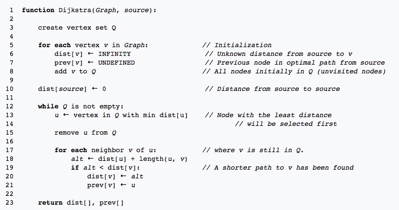
So here is the pseudocode for the Shortest-Path Algorithm, thanks to Wikipedia:

Walking through the Pseudocode

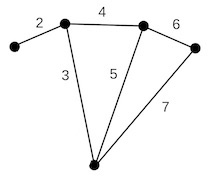
So let's walk through this cryptic pseudocode thing! Lines 5-8 tell us to create a table like the one shown here to start:

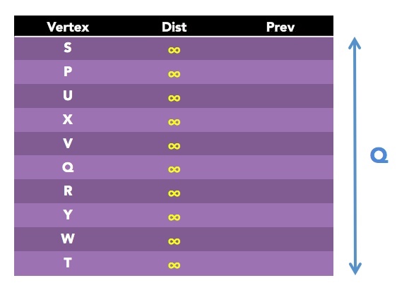
The vertex set Q will start with all vertices in the graph, as indicated by the arrow range on the right.

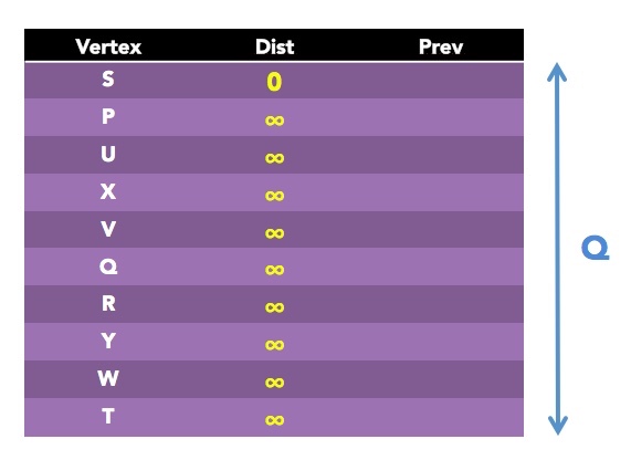
Line 10 says to set Dist (short for "distance from the source vertex S") to 0. That makes sense. The distance from S to S is 0. So let's update our table:

In line 12, the while command is telling us to keep repeating the process in lines 13-21, as long as the set Q is not empty. Since it's currently not, let's jump in there!

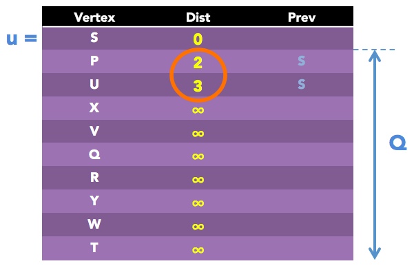
Line 13 says to pick variable u to be a vertex in Q with smallest Dist. Looking at our table, it is obvious that u should be set to S, since it has Dist = 0, while others are infinity.

Line 15 will tell us to now remove S from Q. Lines 17-21 are saying go through the neighbors of u (which is now S). For each one (call it v), we should set a new variable alt to be Dist value of u, plus distance between vertices u and v.

OK! So S has two neighbors: P and U. Let's do v = P first:

alt = Dist of S + distance(S, P) = 0 + 2 = 2

Line 19 says, if this value is less than current Dist value of v (which it is, because the current value of P is infinity) then set it to this new value, and also set Prev value of v (which is P) to u (which is S).

And now for v = U:

alt = Dist of S + distance(S, U) = 0 + 3 = 3

Line 19 says, if this value is less than current Dist value of v (which it is, because the current value of U is infinity) then set it to this new value, and also set Prev value of v (which is U) to u (which is S).

The resulting table will look like this:

Now that we have finished an iteration of the loop, it is time to check if we are done or need to repeat. Line 12 says repeat as long as Q is not empty. Because our Q is not empty, we'll repeat, restarting at line 13.

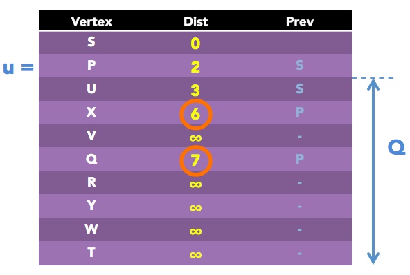
Line 13 says to assign the variable u the vertex in the set Q with the minimum Dist value, which happens to be P with a Dist value of 2. So let's set u = P

Repeating the process, we now look at neighbors of P contained in Q, which are X and Q:

Let's do v = X first:

alt = Dist of P + distance(P, X) = 2 + 4 = 6

Line 19 says, if this value is less than current Dist value of v (which it is, because the current value of X is infinity) then set it to this new value, and also set Prev value of v (which is X) to u (which is P).

And now for v = Q first:

alt = Dist of P + distance(P, Q) = 2 + 5 = 7

Line 19 says, if this value is less than current Dist value of v (which it is, because the current value of Q is infinity) then set it to this new value, and also set Prev value of v (which is Q) to u (which is P). So our updated table looks as follows.

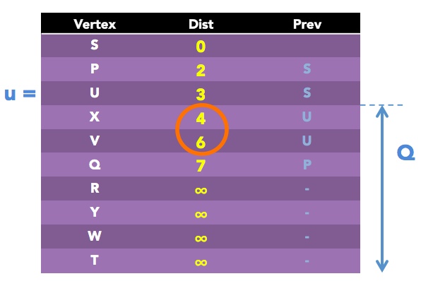
Next round. minimum Dist value is within Q vertices is that of U, so we set u = U.

It' neighbors, which remain in Q, are X and V.

Let's do v = X first:

alt = Dist of U + distance(U, X) = 3 + 1 = 4

Line 19 says, if this value is less than current Dist value of v (which it is, because Dist value for X is 6 at the moment) then set it to this new value, and also set Prev value of v (which is X) to u (which is U).

Now for v = V:

alt = Dist of U + distance(U, V) = 3 + 3 = 6

Line 19 says, if this value is less than current Dist value of v (which it is, because Dist value for X is infinity at the moment) then set it to this new value, and also set Prev value of v (which is V) to u (which is U).

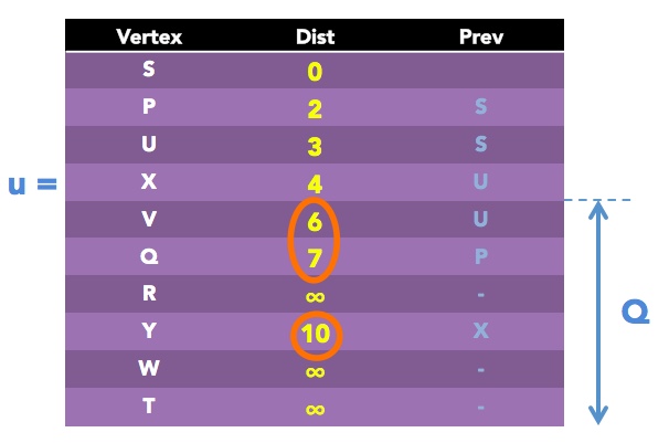
Again, we have to repeat the loop, this time for u = X, since it has a Dist value of 4, least of all others remaining in Q. It has remaining neighbors Q, V and Y.

Let's do v = Q first:

alt = Dist of X + distance(X, Q) = 4 + 7 = 11

Line 19 says, if this value is less than current Dist value of v then update it. However, notice that current Dist value of Q is 7. But because 11 > 7 we don't make any updates to its Dist or Prev values!

Now for v = V:

alt = Dist of X + distance(X, V) = 4 + 8 = 12

Again, current Dist value of V is 6. And since 12 > 6 we don't make any updates to its Dist or Prev values.

Now for v = Y:

alt = Dist of X + distance(X, Y) = 4 + 6 = 10

Since current Dist value of Y is infinity, and 10 < infinity, then we will make set Dist of Y = 10 and Prev of Y = X.

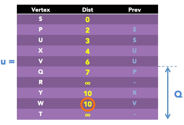
In the next round, we would have to set u = V, since it has the smallest Dist value currently. This vertex has only one neighbor v = W which still remains in Q.

alt = Dist of V + distance(V, W) = 6 + 4 = 10

Since current Dist value of X is infinity, and 10 < infinity, then we will make set Dist of W = 10 and Prev of W = X:

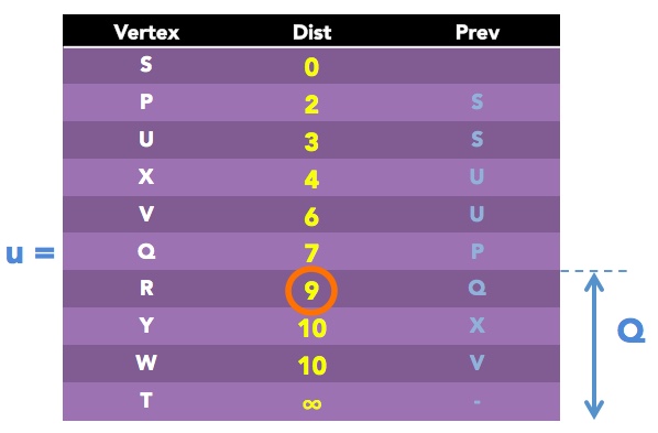
Next, we set u = Q, since it has the smallest Dist value of 7 currently. This vertex has only one neighbor v = R which still remains in Q.

alt = Dist of Q + distance(Q, R) = 7 + 2 = 9

Since current Dist value of R is infinity, and 9 < infinity, then we will make set Dist of Q = 9 and Prev of Q = Q:

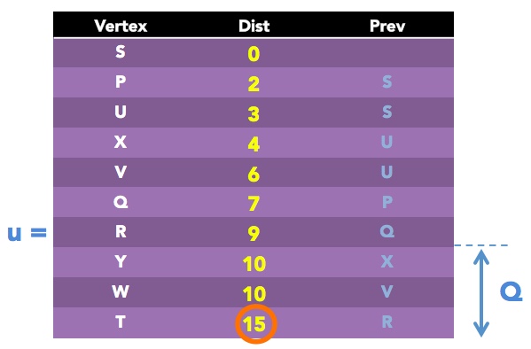
Next, we set u = R, since it has the smallest Dist value of 9 currently. This vertex has only two neighbors Y and Twhich still remains in Q.

Let's start with v = T:

alt = Dist of R + distance(R, T) = 9 + 6 = 15

Since current Dist value of T is infinity, and 15 < infinity, then we will make set Dist of T = 15 and Prev of T = R.

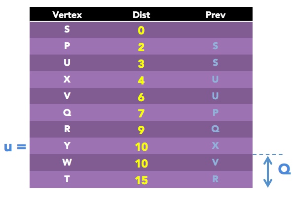
And now for v = Y:

alt = Dist of R + distance(R, Y) = 9 + 1 = 10

Since current Dist value of T is 10, and alt = 10 is not less than 10, then we will not update anything for this vertex.

Now for our next loop, we have two vertices with minimum Dist values, since there are 2 10s out there. So we can just pick any of the two as the next u. Say we pick u = Y. It has only the neighbor v = W among vertices that remain in Q.

alt = Dist of Y + distance(Y, W) = 10 + 3 = 13

Since alt = 13 is not less than the current Dist value of W which is 10, we will not update anything for this vertex.

Next we pick u = W, since its Dist is less than the only other remaining vertex T. For its only remaining neighbor v = T:

alt = Dist of W + distance(W, T) = 10 + 5 = 15

Since alt = 15 is not less than the current Dist value of T which is 15, we will not update anything for this vertex.

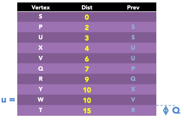
We are finally done with the loop, because only one vertex now remains in Q!

OK. Looking at our complete table, we can now use the Prev values and "backtracking" to find the shortest path between any two vertices!

For example, if we want to know the shortest path from S to T:

Since Prev of T = R, and Prev of R = Q and Prev of Q = P and Prev of P = S, then the shortest path is S-P-Q-R-T.

And since Dist of T = 15, then this shortest path has the total distance of 15.

Boy, that was long! But it was fun, no?! In the next class, we will do a Snap! exercise to implement this algorithm.